15 Excel Formulas, Keyboard Shortcuts & Tricks That'll Save You Lots of Time Excel Formulas The formula: =SUMIF(sum_range, criteria_range1, criteria1, [criteria_range2, criteria2], ...) Sum_range: The range of cells you're going to add up. Scour your data sets to make sure the column of data you're using to combine your information is exactly the same, including no extra spaces. Table Array: The range of columns on Sheet 2 you're going to pull your data from, including the column of data identical to your lookup value (in our example, email addresses) in Sheet 1 as well as the column of data you're trying to copy to Sheet 1. There are times when we want to know how many times a value appears in our spreadsheets. Formula in below example: =IF(D2="Gryffindor","10","0") top: The highest number in the range, Formula in below example: =RANDBETWEEN(1,10) Excel Keyboard Shortcuts 7) Quickly select rows, columns, or the whole spreadsheet. Start by selecting the cell to which you want to add this information. If you've got a ton of different sheets in one workbook -- which happens to the best of us -- make it easier to identify where you need to go by color-coding the tabs. When you want to make a note or add a comment to a specific cell within a worksheet, simply right-click the cell you want to comment on, then click Insert Comment.

To help you use Excel more effectively (and save a ton of time), we’ve compiled a list of essential functions, keyboard shortcuts, and other small tricks you should know.
15 Excel Formulas, Keyboard Shortcuts & Tricks That’ll Save You Lots of Time
Excel Formulas
1) SUMIF
Let’s say you want to determine the profit you generated from a list of leads who are associated with specific area codes, or calculate the sum of certain employees’ salaries — but only if they fall above the a particular amount. Doing that manually sounds a bit time-consuming, to say the least.
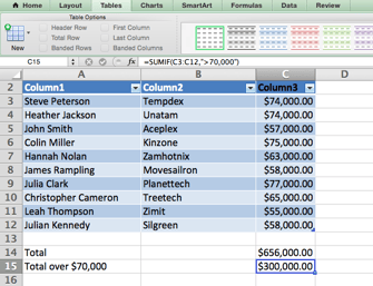
With the SUMIF function, it doesn’t have to be — you can easily add up the sum of cells that meet a certain criteria, like in the salary example above.
- The formula: =SUMIF(sum_range, criteria_range1, criteria1, [criteria_range2, criteria2], …)
- Sum_range: The range of cells you’re going to add up.
- Criteria_range1: The range that is being tested using Criteria1.
- Criteria1: The criteria that determine which cells in Criteria_range1 will be added together.
In the example below, we wanted to calculate the sum of the salaries that were greater than $70,000. The SUMIF function added up the dollar amounts that exceeded that number in the cells C3 through C12, with the formula =SUMIF(C3:C12,”>70,000″).
2) TRIM
Email and file sharing are wonderful tools in today’s workplace. That is, until one of your colleagues sends you a worksheet with some really funky spacing. Not only can those rogue spaces make it difficult to search for data, but they also affect the results when you try to add up columns of numbers.
Rather than painstakingly removing and adding spaces as needed, you can clean up any irregular spacing using the TRIM function, which is used to remove extra spaces from data (except for single spaces between words).
- The formula: =TRIM(“Text”)
- Text: The text from which you want to remove spaces.
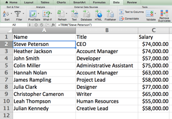
Here’s an example of how we used the TRIM function to remove extra spaces after a name on our list. To do so, we entered =TRIM(“Steve Peterson”) into the Formula Bar.
3) LEFT, MID, and RIGHT
Let’s say you have a line of text within a cell that you want to break down into a few different segments. Rather than manually retyping each piece of the code into its respective column, users can leverage a series of string functions to deconstruct the sequence as needed: LEFT, MID, or RIGHT.
LEFT:
- Purpose: Used to extract the first X numbers or characters in a cell.
- The formula: =LEFT(text, number_of_characters)
- Text: The string that you wish to extract from.
- Number_of_characters: The number of characters that you wish to extract starting from the left-most character.
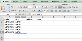
In the example below, we entered =LEFT(A2,4) into cell B2, and copied it into B3:B6. That allowed us to extract the first 4 characters of the code.
MID:
- Purpose: Used to extract characters or numbers in the middle based on position.
- The formula: =MID(text, start_position, number_of_characters)
- Text: The string that you wish to extract from.
- Start_position: The position in the string that you want to begin extracting from. For example, the first position in the string is 1.
- Number_of_characters: The number of characters that you wish to extract.
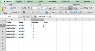
In this example, we entered =MID(A2,5,2) into cell B2, and copied it into B3:B6. That allowed us to extract the two numbers starting in the fifth position of the code.
RIGHT:
- Purpose: Used to extract the last X numbers or characters in a cell.
- The formula: =RIGHT(text, number_of_characters)
- Text: The string that you wish to extract from.
- Number_of_characters: The number of characters that you want to extract starting from the right-most character.
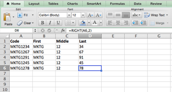
For the sake of this example, we entered =RIGHT(A2,2) into cell B2, and copied it into B3:B6. That allowed us to extract the last two numbers of the code.
4) VLOOKUP
This one is an oldie, but a goodie — and it’s a bit more in depth than some of the other formulas we’ve listed here. But it’s especially helpful for those times when you have two sets of data on two different spreadsheets, and want to combine them into a single spreadsheet.
My colleague, Rachel Sprung — whose “How to Use Excel” tutorial is a must-read for anyone who wants to learn — uses a list of names, email addresses, and companies as an example. If you have a list of people’s names next to their email addresses in one spreadsheet, and a list of those same people’s email addresses next to their company names in the other, but you want the names, email addresses, and company names of those people to appear in one place — that’s where VLOOKUP comes in.
Note: When using this formula, you must be certain that at least one column appears identically in both spreadsheets. Scour your data sets to make sure the column of data you’re using to combine your information is exactly the same, including no extra spaces.
- The formula: VLOOKUP(lookup value, table array, column number, [range lookup])
- Lookup Value: The identical value you have in both spreadsheets. Choose the first value in your first spreadsheet. In Sprung’s example that follows, this means the first email address on the list, or cell 2 (C2).
- Table Array: The range of columns on Sheet 2 you’re going to pull your data from, including the column of data identical to your lookup value (in our example, email addresses) in Sheet 1 as well as the column of data you’re trying to copy to Sheet 1. In our example, this is “Sheet2!A:B.” “A” means Column A in Sheet 2, which is the column in Sheet 2 where the data identical to our lookup value (email) in Sheet 1 is listed. The “B” means Column B, which contains the information that’s only available in Sheet 2 that you want to translate to Sheet 1.
- Column Number: The table array tells Excel where (which column) the new data you want to copy to Sheet 1 is located. In our example, this would be the “House” column, the second one in our table array, making it column number 2.
- Range Lookup: Use FALSE to ensure you pull in only exact value matches.
- The formula with variables from Sprung’s example below: =VLOOKUP(C2,Sheet2!A:B,2,FALSE)
In this example, Sheet 1 and Sheet…
COMMENTS